Eophis Tutorial
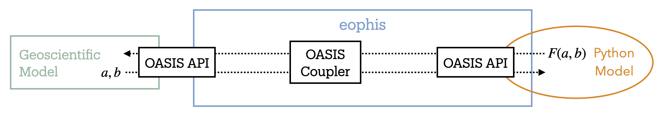
In this tutorial we will build the Eophis script to couple a Forcing Model with a geophysical code.
- Prerequisites to the tutorial:
Installed Eophis package - we strongly recommand installation From Container
Introduction
A surrogate geoscientific model “Toy Earth” with an OASIS interface is emulated by toy_earth_tuto.py. It initializes three dimensionless physical 3D fields U, V, T, discretized on metric 2D fields X, Y that represent the simulated domain. The script advances in time in accordance with parameters provided in the fortran namelist earth_namelist_tuto and updates the physical fields with the following equation:
A = A + dt**2 / 100. * B
Where A is one of the abovementioned physical fields and B a forcing term corresponding to A.
- The model can be executed in two distinct modes:
standalone:
Bis imposed with a constant value. OASIS interface is disabled.coupled: OASIS interface is activated and Toy Earth can send the physical and metric fields through OASIS. It can also receive up to three forcing fields. If a forcing field is received, it is used instead of
Bfor time advancement.
Note
It is then possible to change the way the physical fields are forced. The only condition is to compute the forcing terms in an external script and to exchange results through OASIS.
Run Toy Earth
We start the tutorial by running Toy Earth in standalone mode. Go in tutorial directory:
cd ~/eophis/tuto
Edit earth_namelist_tuto to create a domain on a 100x100 grid with three levels on third dimension. Set the time configuration to run the model on one hundred time steps of five seconds.
vi earth_namelist_tuto
nn_it000   =   1
nn_itend   = 101
# ...
rn_Dt = 5
nlon = 100
nlat = 100
nlvl = 3
Beware to keep ln_cpl = .false. to run the model lonely. Toy Earth is also able to plot the physical fields all along the run, set the output frequency as follows:
vi earth_namelist_tuto
nn_write   =  25
Now run Toy Earth:
python3 ./toy_earth_tuto.py
# NB: Toy Earth is parallelized
mpirun -np 2 python3 ./toy_earth_tuto.py
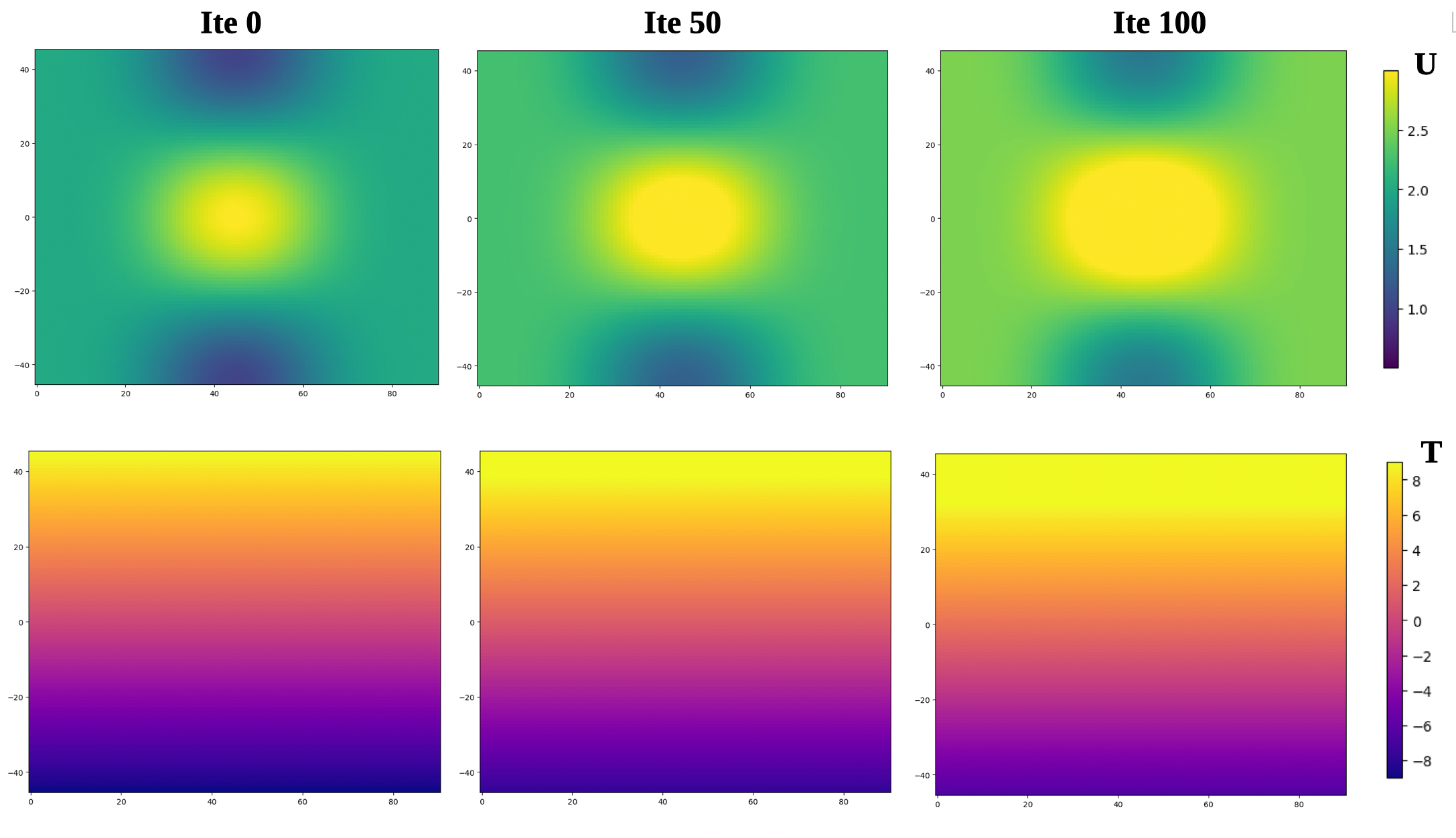
You should find some color maps named with the following convention <field-name>_<output-iteration>.png. They show the evolution of the physical fields computed by the model (first level only).
Field values slowly increase due to the uniform constant forcing term.
You can also check out content of earth.log.
Run Forcing Model
We wish a different forcing term for U. For the tutorial we will use dU/dX. As described earlier, the forcing term must be computed in an external script. Edit models_tuto.py, an empty function compute_gradient() is already defined. Complete content of function structure to compute the gradient of an array dat against an array x in the first dimension:
def compute_gradient(dat,x):
    """ Compute gradient of dat (numpy.ndarray) against x (numpy.ndarray) """
    if Is_None(dat,x):
        return None
    else:
        ddat = np.gradient(dat,axis=0)
        dx = np.gradient(x,axis=0)
        return ddat / dx
Note that in accordance with header instructions, compute_gradient() returns None if at least one of the inputs is None. models_tuto.py can be executed as a standalone script. Run it to check that the Forcing Model works correctly:
python3 ./models_tuto.py
# Should print:
#   Returned forcing shape: (50,25,10)
#   Test successful
Note
We have now an external forcing model we wish our geoscientific code to use. However, models_tuto.py does not possess an OASIS interface and cannot be coupled with Toy Earth. In the next sections, we will build the Eophis script to set up and configure the coupling environment.
Eophis Script
Some material and information are required to set up the coupling. We will generate everything with the Eophis script eophis_script_tuto.py. The script may execute preproduction() or production(). The first function is used to generate coupling material. The second one contains instructions to perform the coupling itself. For both, we need to define what we want to exchange in toy_earth_info().
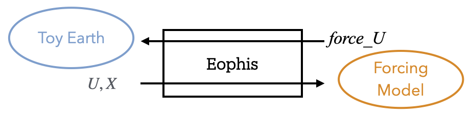
Defining the exchanges
- Toy Earth needs to send:
whole field
U, at each time step as it evolves, on 3D grid(100,100,3)whole field
X, only once as it is fixed, on 2D grid(100,100)
- and to receive from Forcing Model:
forcing field
force_U, at each time step, on 3D grid(100,100,3)
In Eophis, exchanges are defined in Tunnel object. Define an empty Tunnel named TO_EARTH (step 1) with:
tunnel_config = list()
tunnel_config.append( { 'label' : 'TO_EARTH', \
                        'grids' : {}, \
                        'exchs' : [ {} ] }
                    )
We now define the grid on which we want to perform the exchanges (i.e. Toy Earth grid):
tunnel_config = list()
tunnel_config.append( { 'label' : 'TO_EARTH', \
                        'grids' : { 'grid_tuto' : {'npts' : (100,100)} }, \
                        'exchs' : [ {} ] }
                    )
What remains now is to define the exchanges themselves. Following Tunnel documentation, we can complete exchanges definition in Tunnel for U, force_U, and X with:
tunnel_config = list()
tunnel_config.append( { 'label' : 'TO_EARTH', \
                        'grids' : { 'grid_tuto' : {'npts' : (100,100)} }, \
                        'exchs' : [ {'freq' : 5, 'grd' : 'grid_tuto' , 'lvl' : 3, 'in' : ['U'], 'out' : ['force_U'] }, \
                                    {'freq' : Freqs.STATIC, 'grd' : 'grid_tuto' , 'lvl' : 1, 'in' : ['X'], 'out' : [] } ] }
                    )
Now that we have defined the exchanges, we can create the Tunnel object in the preproduction() function (step 4) with:
to_earth, = eophis.register_tunnels( tunnel_config )
Eophis is now aware of the exchanges to perform with OASIS.
Generate OASIS material
OASIS namelist can be generated with write_coupling_namelist(). This function requires total simulation time as argument. This information is available from time parameters in Toy Earth namelist. Define a Fortran Namelist object (step 2) from earth_namelist_tuto with:
earth_nml = eophis.FortranNamelist(os.path.join(os.getcwd(),'earth_namelist_tuto'))
and read parameters (step 3) with:
step, it_end, it_0 = earth_nml.get('rn_Dt','nn_itend','nn_it000')
total_time = (it_end - it_0 + 1) * step
We finally generate OASIS namelist (step 5) with:
eophis.write_coupling_namelist( simulation_time=total_time )
Eophis preproduction script is now ready to be executed:
python3 ./eophis_script_tuto.py --exec preprod
We have generated three files: Eophis logs eophis.out, eophis.err, and namelist namcouple. The latter is required by OASIS, do no remove it (or rerun Eophis preproduction script).
Configure Toy Earth
Now we configure coupling from Toy Earth side. Toy Earth needs to know the names under which OASIS will manipulate the variables to exchange. This information is available in eophis.log:
cat eophis.out
# [...]
========= EOPHIS TUTO : Pre-Production =========
  Aim: write coupling namelist

-------- Tunnel TO_EARTH registered --------
  namcouple variable names
    Earth side:
      - U -> E_OUT_0
      - force_U -> E_IN_0
      - X -> E_OUT_1
    Models side:
      - U -> M_IN_0
      - force_U -> M_OUT_0
      - X -> M_IN_1
We can see here that U, force_U, and X are manipulated by OASIS under E_OUT_0, E_IN_0, and E_OUT_1, respectively. In accordance with these informations, edit earth_namelist_tuto as follows to switch Toy Earth to coupled mode:
vi earth_namelist_tuto
ln_cpl = .true.
!         !  Variable name  ! couple variable (T/F) ! OASIS namcouple name ! number of levels !
cpl_u =           'U'       ,        .true.         ,       'E_OUT_0'      ,        3
cpl_v =           'V'       ,        .false.        ,         '...'        ,       ...
cpl_t =           'T'       ,        .false.        ,         '...'        ,       ...
cpl_x =           'X'       ,        .true.         ,       'E_OUT_1'      ,        1
cpl_y =           'Y'       ,        .false.        ,         '...'        ,       ...
! ------- !
cpl_force_u  =  'force_U'   ,        .true.         ,       'E_IN_0'       ,        3
cpl_force_v  =  'force_V'   ,        .false.        ,         '...'        ,       ...
cpl_force_t  =  'force_T'   ,        .false.        ,         '...'        ,       ...
Connect models
We build now the production() function that will deploy the OASIS interface in models_tuto.py and drive the exchanges all along the run. With the exchanges defined in the registered Tunnel and the runtime information from the Fortran namelist, we have all the necessary material to start coupling. We can deploy the OASIS interface (step 6) using:
eophis.open_tunnels()
Coupling is now effective and we can perform exchanges with Tunnel. During preproduction phase, we defined a static exchange for X. This means that receiving X must be performed manually before to start any time-automated exchanges. Now that OASIS is activated, we can receive X (step 7) with help of this Tunnel method:
x = to_earth.receive('X')
We will use x as argument for the Forcing Model. We import it (step 8):
from models_tuto import compute_gradient
U field is still missing to call Forcing Model. During preproduction, we identified that exchanges of U and force_U should be repeated in time. Synchronization of exchanges in time is done by Loop. Loop requires a Tunnel to work with, number of time iteration, and time step value. Define Loop (step 9) as follows:
@eophis.all_in_all_out( geo_model=to_earth, step=step, niter=niter )
Final step is to specify connexions between the exchanged data and the Forcing Model. Edit content of loop_core() as follows:
def loop_core(**inputs):
    """
    Loop is defined with the decorator and time step information from 'earth_namelist_tuto'.
    Content of loop_core is the Router. Connexions between exchanged variables and models are defined here.
    inputs dictionary contains the variables that Eophis automatically received from toy_earth_tuto.py through OASIS.

    """
    outputs = {}
    outputs['force_U'] = compute_gradient( inputs['U'], x )
    return outputs
Note that everything is assembled here. We are now ready to run Toy Earth in coupled mode:
mpirun -np 1 python3 ./toy_earth_tuto.py : -np 1 python3 ./eophis_script_tuto.py
We can see that new forcing makes U field to evolve differently in time.
Parallel execution
Tutorial grid is small. For bigger grid size, it can be necessary to share work on several processes. Good news is that Eophis is parallelized, let’s give a try:
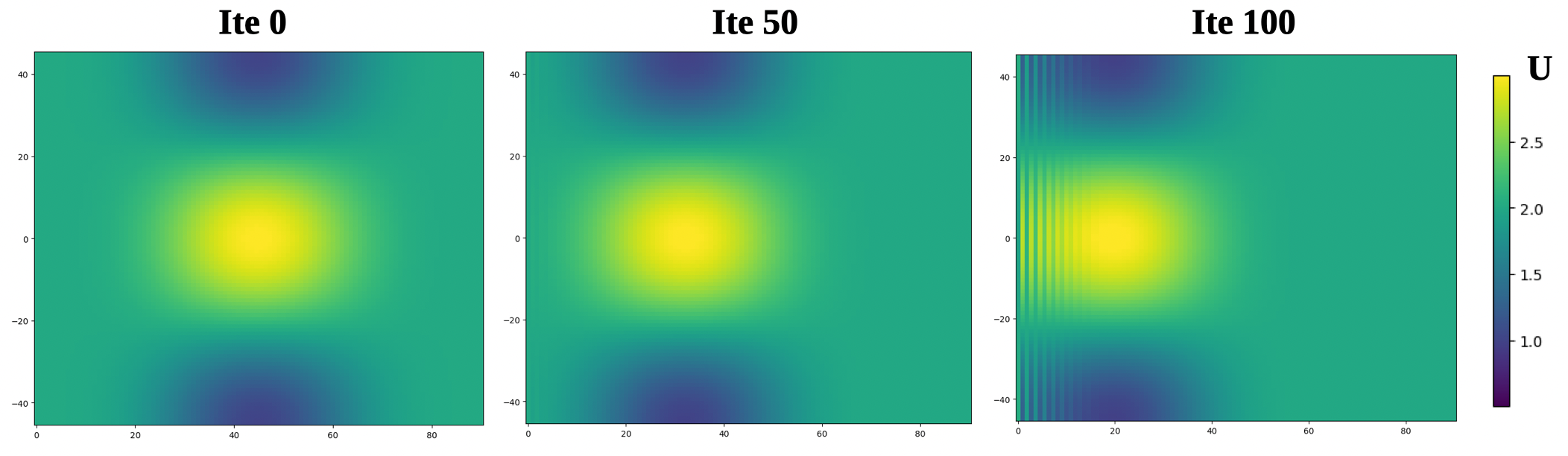
mpirun -np 1 python3 ./toy_earth_tuto.py : -np 5 python3 ./eophis_script_tuto.py
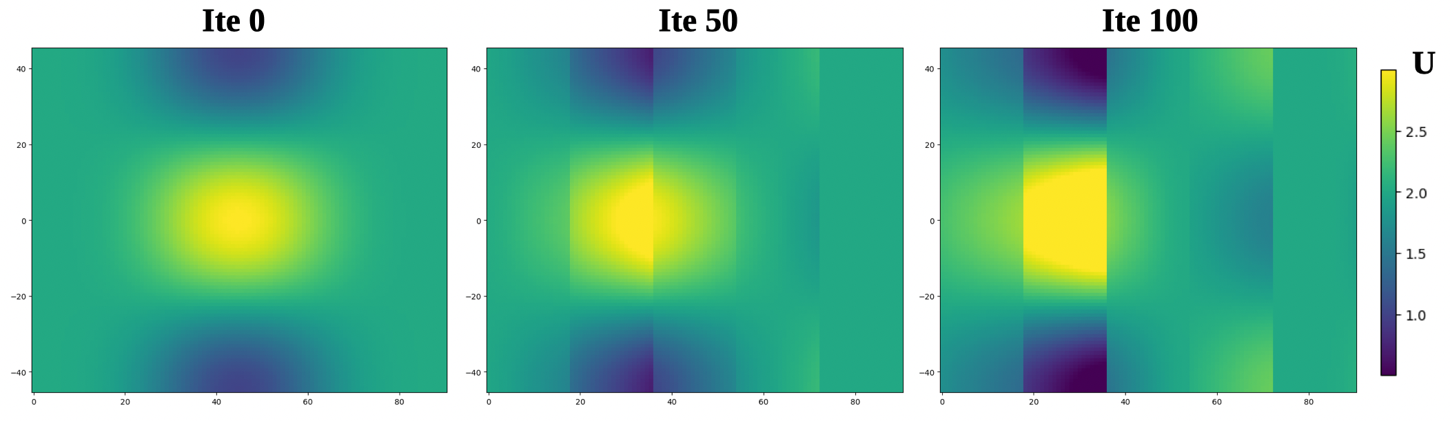
There is somethong wrong here: the evolution of U has deteriorated. This is because U and X fields are distributed among Eophis processes, and edge effects appear when computing the gradient near internal boundaries. The five subdomains can indeed be distinguished in the color map.
This problem could be overcome if Eophis processes had access to the values of neighboring subdomains grid cells . By default, numpy.gradient() in models_tuto.py uses first-order finite differences at the edges. In this case, just one extra cell would be sufficient.
It is possible to configure Eophis to create extra halos cells when exchanging fields with coupled geophysical model. These halos cells will be available when receiving fields and ignored when sending them back. Edit eophis_script_tuto.py and adapt the grid definition in Tunnel as follows:
# Grid without halos
'grids' : { 'grid_tuto' : {'npts' : (100,100)} }, \
# New grid with halos
'grids' : { 'grid_tuto' : {'npts' : (100,100), 'halos' : 1} }, \
We need to specify what values should contain the halo cells outside the edges of the global domain. By default, those halos are set to zero. This is a problem here because gradient at the boundary will exhibit anomalies. A better solution is to fill these extra cells as if the grid were periodic. We adapt one last time the grid definition:
# Periodic boundary conditions
'grids' : { 'grid_tuto' : {'npts' : (100,100), 'halos' : 1, 'bnd' : ('cyclic','cyclic')} }, \
No need to run preproduction script again. Re-run production test case in parallel. Results should now be identical to previous section.
Going further
You have seen main Eophis features for coupling a Python script with a geophysical model. Do no hesitate to check out concepts and usage sections to explore more advanced eophis functionalities. Tests section can also provide inspiration.
Using this documentation, a good exercise would be to set up a coupling where the forcing of U, V, and T follows these advection equations:
force_U = U * dU/dX + V * dU/dY
force_V = U * dV/dX + V * dV/dY
force_T = U * dT/dX + V * dT/dY